Tutorial 6: Modeling Spot Crossings During Transits#
Author: Hannu Parviainen Edited: 5 February 2026
This notebook demonstrates how to model spot crossings during exoplanet transits using ExoIris. When a transiting planet crosses a star spot, it temporarily blocks less light than when crossing the normal stellar surface, creating a characteristic “bump” in the light curve. If left unmodeled, these spot crossings can bias the transmission spectrum.
We will analyze real JWST NIRISS observations of HAT-P-18b that contain a clear spot crossing event, showing how to:
Identify spot crossings in the data
Initialize and configure the spot model
Set appropriate priors for spot parameters
Fit the data with the spot model
Interpret the results
[1]:
%run ../setup_multiprocessing.py
[2]:
from multiprocessing import Pool
from numpy import concatenate
from matplotlib.pyplot import subplots, rc
import astropy.io.fits as pf

from exoiris import ExoIris, TSData
from exoiris.ephemeris import Ephemeris

rc('figure', figsize=(12,4))
Data Loading#
We load JWST NIRISS observations of HAT-P-18b from June 2022, which contain a clear spot crossing event visible in the white light curve. The data comes in two spectral orders: Order 1 covers the longer wavelengths (0.9–2.8 \(\mu\)m) and Order 2 covers the shorter wavelengths (0.62-0.84 \(\mu\)m). The data is pre-binned both in time and wavelength for this example.
[3]:
ephemeris = Ephemeris(59743.352, 5.508029, 0.12)
[4]:
with pf.open('data/hat-p-18b-2022-06-niriss-o1.fits') as hdul:
    d1 = TSData.import_fits('NIRISS-O1', hdul)
    d1.mask_transit(ephemeris=ephemeris)
    d1.estimate_average_uncertainties()
    d1.n_baseline = 1

with pf.open('data/hat-p-18b-2022-06-niriss-o2.fits') as hdul:
    d2 = TSData.import_fits('NIRISS-O2', hdul)
    d2.mask_transit(ephemeris=ephemeris)
    d2.estimate_average_uncertainties()
    d2.n_baseline = 1

d2 = d2.crop_wavelength(0.6, 0.84)
d = d2 + d1
[5]:
fig, axs = subplots(2, 2, figsize=(13, 7), constrained_layout=True)
d.plot(axs=axs[:,0])
d.plot_white(axs=axs[:,1]);
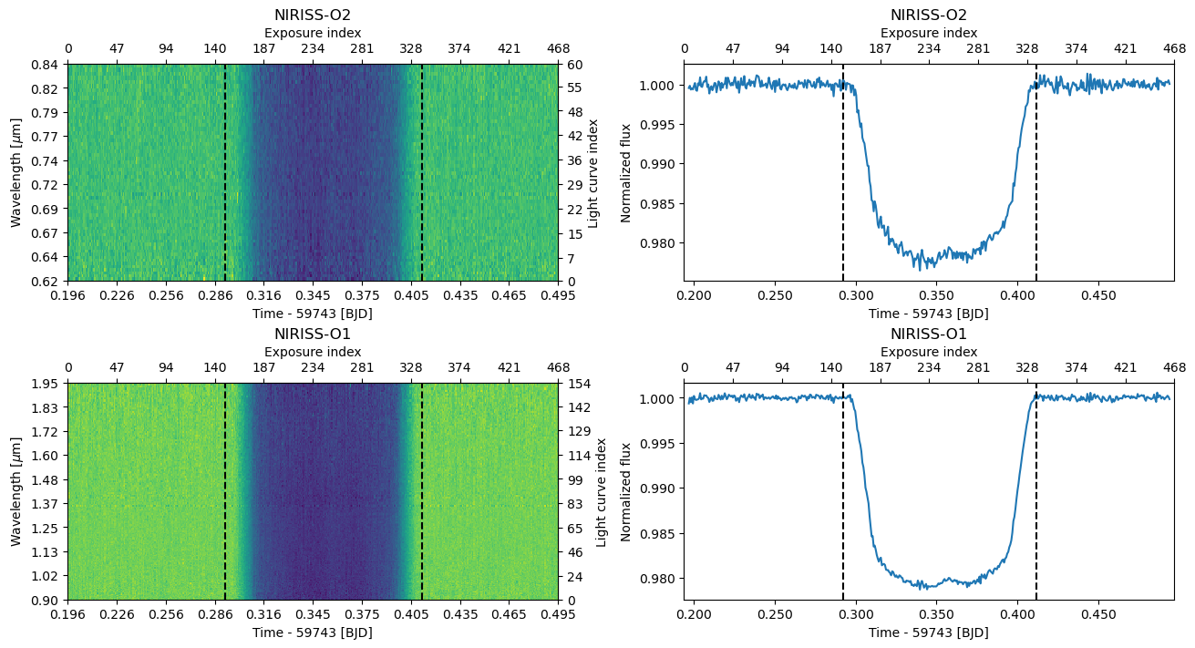
Look at the white light curves on the right. You can see a clear bump during the transit around BJD 59743.355 - this is the spot crossing event we want to model!
Understanding Spot Crossings#
When a planet transits across a cooler star spot, it temporarily blocks less light than when crossing the normal stellar photosphere. This creates a positive “bump” in the light curve during transit. The amplitude and duration of this bump depend on:
Spot size and position: Larger spots create bigger bumps; position determines when during transit the bump appears
Spot temperature: Cooler spots create larger amplitude bumps
Wavelength: The contrast between spot and photosphere is wavelength-dependent, typically stronger at shorter wavelengths
ExoIris models spot crossings using the following parameters:
Parameter |
Name |
Description |
|---|---|---|
|
Center |
Time of maximum spot crossing amplitude |
|
Amplitude |
Maximum flux anomaly at the reference wavelength |
|
FWHM |
Full width at half maximum (duration) of the crossing |
|
Shape |
Shape parameter, where 2 gives a Gaussian |
|
Temperature |
Effective temperature of the spot |
The wavelength-dependent contrast is computed using BT-Settl stellar atmosphere models, so you only need to specify the spot temperature - ExoIris handles the spectral contrast automatically.
Initialize ExoIris with Spot Model#
[6]:
ts = ExoIris('06_spot_crossing', 'power-2', d, nk=50, nthreads=1)
ts.set_prior('tc_00', 'NP', ephemeris.zero_epoch, 0.003)
ts.set_prior('p', 'NP', ephemeris.period, 1e-7)
ts.set_prior('rho', 'NP', 2.68, 0.2)
ts.set_prior('radius ratios', 'UP', 0.125, 0.145)
ts.set_ldtk_prior((4790, 120), (4.58, 0.01), (0.14, 0.1), uncertainty_multiplier=10)
Add the Spot Model#
Now we initialize the spot model and add a spot. The key parameters are:
tstar: Stellar effective temperature (K) - used for contrast calculationswlref: Reference wavelength (\(\mu\)m) where the spot amplitude is definedinclude_tlse: Whether to include Transit Light Source Effect (unocculted spots/faculae)
[7]:
ts.initialize_spots(tstar=4790, wlref=1.5, include_tlse=False)
ts.add_spot(epoch_group=0)
Let’s examine the new spot parameters that have been added to the model:
[8]:
ts.ps[-10:]
[8]:
[ 72 |G| k_01.86618     U(a = 0.125, b = 0.145)                  [    0.00 ..      inf],
  73 |G| k_01.89324     U(a = 0.125, b = 0.145)                  [    0.00 ..      inf],
  74 |G| k_01.92030     U(a = 0.125, b = 0.145)                  [    0.00 ..      inf],
  75 |G| k_01.94735     U(a = 0.125, b = 0.145)                  [    0.00 ..      inf],
  76 |G| sigma_m_00     N(μ = 1.0, σ = 0.01)                     [    0.00 ..      inf],
  77 |G| spc_01         U(a = 0, b = 1)                          [    0.00 ..      inf],
  78 |G| spa_01         U(a = 0, b = 1)                          [    0.00 ..      inf],
  79 |G| spw_01         U(a = 0, b = 1)                          [    0.00 ..      inf],
  80 |G| sps_01         U(a = 1, b = 5)                          [    0.00 ..      inf],
  81 |G| spt_01         U(a = 3000, b = 6000)                    [    0.00 ..      inf]]
Set Spot Priors#
We need to set appropriate priors for the spot parameters based on our visual inspection of the data:
Center time (``spc_01``): The bump appears around BJD 59743.355
Amplitude (``spa_01``): The bump is small, maybe ~0.1% of the flux
FWHM (``spw_01``): The bump lasts roughly 0.01-0.02 days
Temperature (``spt_01``): Spot should be cooler than the star (4790 K)
[9]:
ts.set_prior('spc_01', 'NP', 59743.355, 0.001)  # Normal prior on center time
ts.set_prior('spa_01', 'UP', 0.0, 0.002)        # Uniform prior on amplitude
ts.set_prior('spw_01', 'UP', 0.001, 0.05)       # Uniform prior on FWHM
ts.set_prior('spt_01', 'UP', 3850, 4790)        # Uniform prior on temperature (must be < Tstar)
[10]:
ts.ps[-6:]
[10]:
[ 76 |G| sigma_m_00     N(μ = 1.0, σ = 0.01)                     [    0.00 ..      inf],
  77 |G| spc_01         N(μ = 59743.355, σ = 0.001)              [    0.00 ..      inf],
  78 |G| spa_01         U(a = 0.0, b = 0.002)                    [    0.00 ..      inf],
  79 |G| spw_01         U(a = 0.001, b = 0.05)                   [    0.00 ..      inf],
  80 |G| sps_01         U(a = 1, b = 5)                          [    0.00 ..      inf],
  81 |G| spt_01         U(a = 3850, b = 4790)                    [    0.00 ..      inf]]
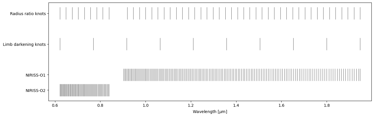
Let’s visualize the model setup including the radius ratio and limb darkening knots:
[11]:
knots = ts.k_knots.copy()
m = (knots > ts.data[0].bbox_wl[1]) & (knots < ts.data[1].bbox_wl[0])
ts.set_radius_ratio_knots(knots[~m])

ts.plot_setup(figsize=(13, 4));
Fitting the Model#
Fit the White Light Curve#
We start by fitting the white light curve to obtain initial estimates of the orbital and planetary parameters. Note that the white light curve fit doesn’t include the spot model.
[12]:
ts.fit_white()
ts.plot_white(figsize=(13, 4));
Set Up Multiprocessing#
[13]:
def lnpostf(pv):
    return ts.lnposterior(pv)

pool = Pool(8)
Global Optimization#
[14]:
ts.fit(niter=5000, npop=200, pool=pool, lnpost=lnpostf)
[15]:
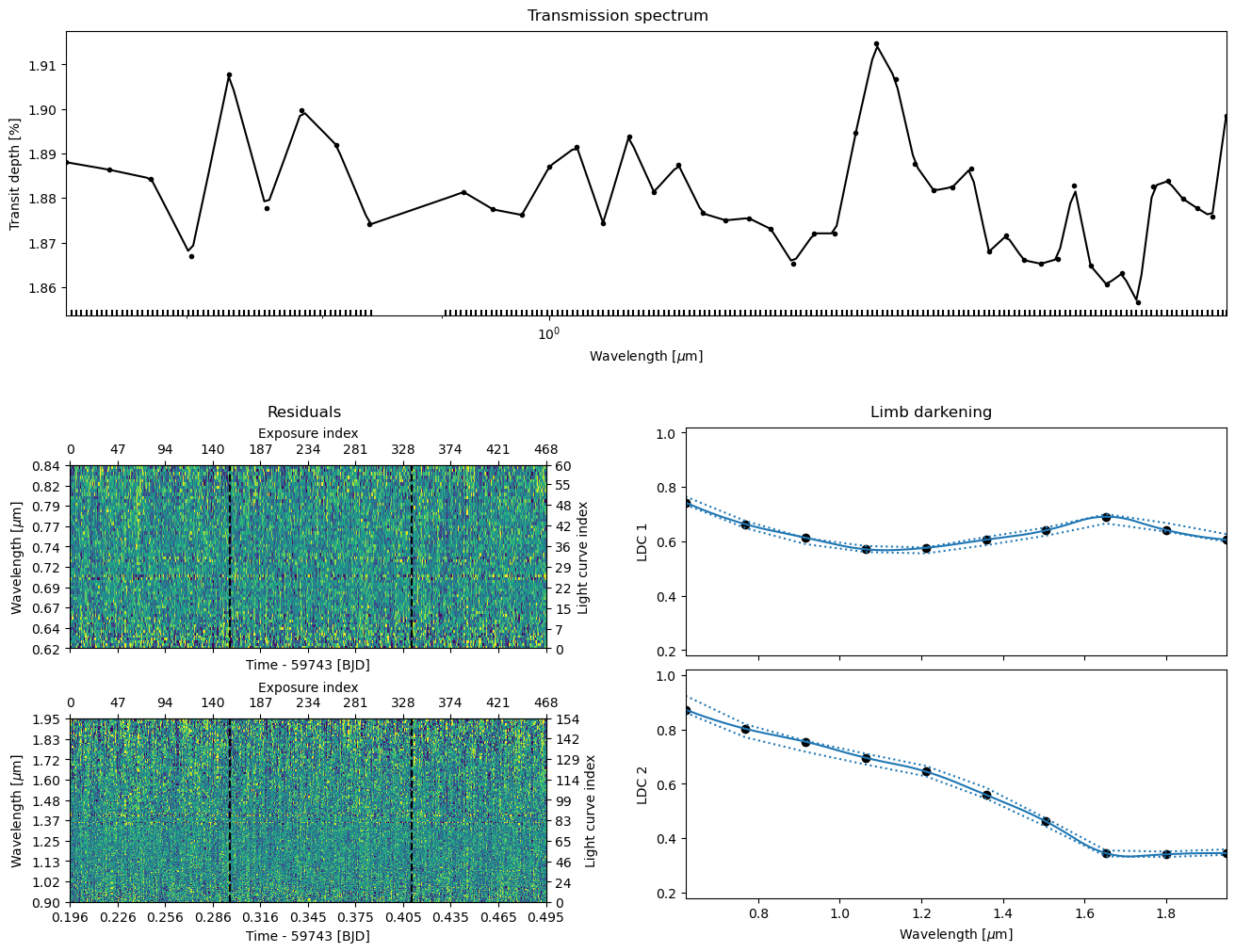
ts.plot_fit(figsize=(13, 10), height_ratios=(1, 1.5), trs_args={'xscale': 'log'});
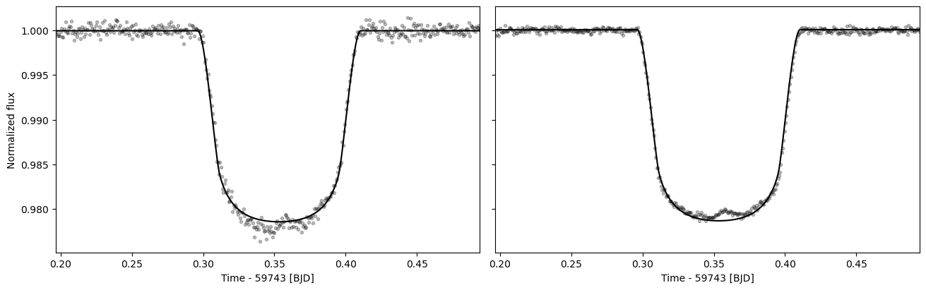
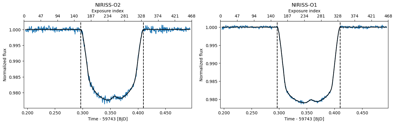
[16]:
mtr = ts._tsa.flux_model(ts._tsa.de.minimum_location, include_baseline=False)

fig, axs = subplots(1, 2, figsize=(13, 4), constrained_layout=True)
for i in range(2):
    ts.data[i].plot_white(ax=axs[i])
    axs[i].plot(ts.data[i].time, ts.data[i].create_white_light_curve(mtr[i][0]), 'k')
MCMC Sampling#
With a good optimization result, we can now run MCMC to obtain posterior samples.
[19]:
ts.sample(1000, thin=50, repeats=3, pool=pool, lnpost=lnpostf)
[20]:
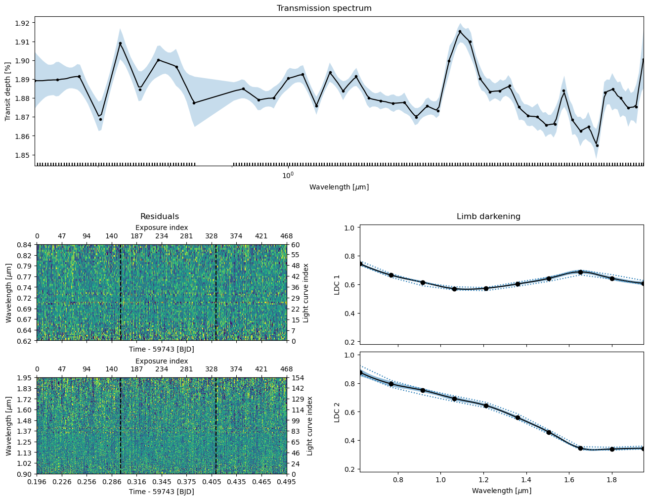
ts.plot_fit('mcmc', figsize=(13, 10), height_ratios=(1, 1.5), trs_args={'xscale': 'log'});
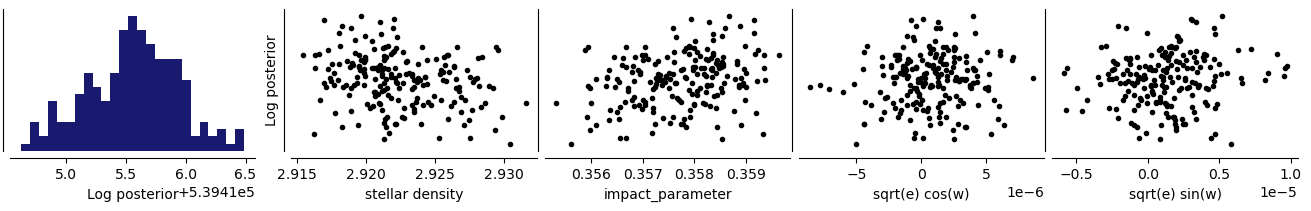
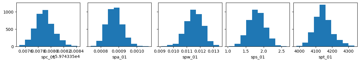
Spot Parameter Posteriors#
Let’s examine the posterior distributions for the spot parameters.
[21]:
spot_cols = [c for c in ts.posterior_samples.columns if c.startswith('sp')]
fig, axs = subplots(1, len(spot_cols), figsize=(12, 2), constrained_layout=True, sharey='all')
for i, ax in enumerate(axs):
    ax.hist(ts.posterior_samples[spot_cols[i]])
    ax.set_xlabel(spot_cols[i])
Save and Cleanup#
[22]:
ts.save(overwrite=True)
[23]:
pool.close()
©2026 Hannu Parviainen