Tutorial 1: The (Not So) Short Introduction to ExoIris

Tutorial 1: The (Not So) Short Introduction to ExoIris#

Author: Hannu Parviainen Edited: 5 February 2026

This notebook gives a rather verbose introduction to transmission spectroscopy with ExoIris and shows how to reproduce a low-resolution version of the transmission spectroscopy analysis of WASP-39b observed with JWST NIRISS by Feinstein et al. (2023). Later notebooks show how to use the LDTk-based limb darkening model and what happens when we increase the resolution.

Note: If you’re looking for a template to start your own analysis with, the The (Very) Short Introduction to ExoIris notebook reproduces this one in a less verbose format.

We start by forcing different multithreaded codes to use a single thread. This is important when parallelising the computations with multiprocessing since it would be very easy to end up with a number of processes all trying to use all the computer’s cores. After this, we initialise Matplotlib and import some standard packages and functions.

[2]:

import os
os.environ["OMP_NUM_THREADS"] =        "1"
os.environ["OPENBLAS_NUM_THREADS"] =   "1"
os.environ["MKL_NUM_THREADS"] =        "1"
os.environ["VECLIB_MAXIMUM_THREADS"] = "1"
os.environ["NUMEXPR_NUM_THREADS"] =    "1"

# I'm forcing the multiprocessing start method to 'fork' on Macs
# because 'spawn' seems to cause errors with the numba code.
from sys import platform
if 'darwin' in platform:
    import multiprocessing as mp
    mp.set_start_method('fork')
else:
    import multiprocessing as mp
    mp.set_start_method('fork')

from numba import set_num_threads, config
config.THREADING_LAYER = 'safe'
set_num_threads(1)

[3]:

from multiprocessing import Pool
from xarray import load_dataset
from scipy.interpolate import splev, splrep
from numpy import array, geomspace, linspace, concatenate, r_
from matplotlib.pyplot import subplots, setp, rc

from exoiris import ExoIris, TSData

[4]:

rc('figure', figsize=(12,4))

Data preparation#

Read in the data#

We read the spectroscopic light curves and store them as exoiris.TSData objects. TSData is an utility class to store and manipulate spectroscopic time series before using them in a transmission spectrum analysis.

None: appendix 1 notebook shows how the original Feinstein et al (2023) light curves downloaded from Zotero are converted into a simple xarray dataset.

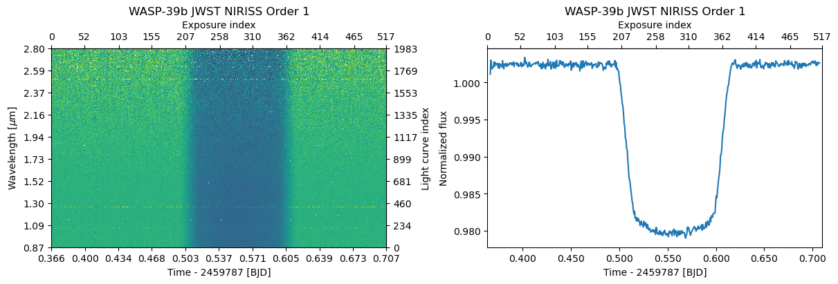
We first define a simple utility function to read the xarray DataSet into TSData and then read the order 1 light curves. We mask any strong individual outlier points, and plot the data.

[5]:

def read_data(fname, name="", noise_group: str = 'a', n_baseline: int = 5):
    with load_dataset(fname) as ds:
        return TSData(time=ds.time.values, wavelength=ds.wavelength.values, fluxes=ds.flux.values, errors=ds.error.values,
                      name=name, noise_group=noise_group, n_baseline=n_baseline)

[6]:

d1 = read_data('data/nirHiss_order_1.h5', "WASP-39b JWST NIRISS Order 1", noise_group=0, n_baseline=1)
d1.crop_wavelength(0.86, 2.8)
d1.mask_outliers(8)

fig, axs = subplots(1, 2, constrained_layout=True)
d1.plot(ax=axs[0])
d1.plot_white(ax=axs[1]);

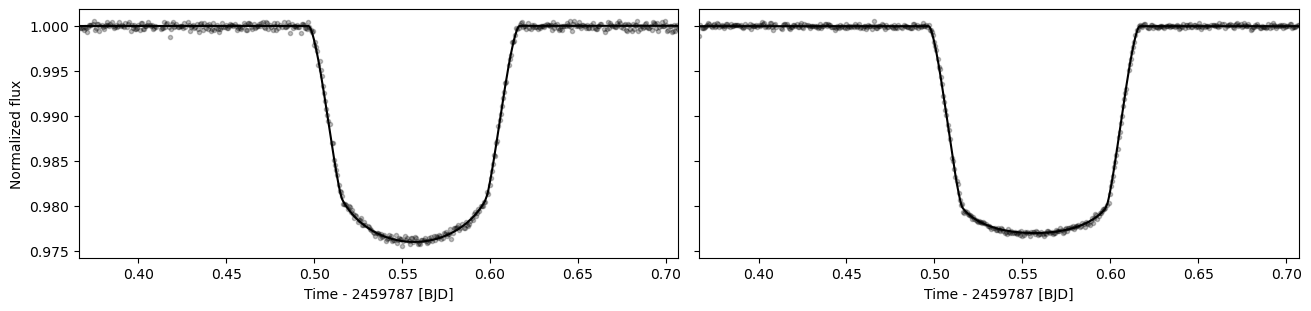
../../_images/examples_e01_01a_not_so_short_intro_6_0.png

Next, we set the transit mask using the TSData.mask_transit method and normalise the spectrophotometric light curves to a line fitted to the the out-of-transit data using the TSData.normalize_to_poly method. We can also normalise the data after the white-light-curve fit, but it is better to do this already here if we’re planning to bin the data along the wavelength-axis, because otherwise the binned data will contain the baseline variations from one light curve to another.

[7]:

d1.mask_transit(t0=2459783.5015, p=4.0552842, t14=0.13)
d1.normalize_to_poly()

fig, axs = subplots(1, 2, constrained_layout=True)
d1.plot(ax=axs[0])
d1.plot_white(ax=axs[1]);

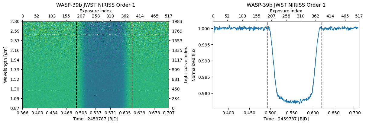
../../_images/examples_e01_01a_not_so_short_intro_8_0.png

The TSData.mask_transit method calculates an out-of-transit mask and stores it in TSData.ootmask. The method also creates an Ephemeris object that is stored in TSData.ephemeris.

[8]:

d1.ephemeris

[8]:

Ephemeris(zero_epoch=2459783.5015, period=4.0552842, duration=0.13)

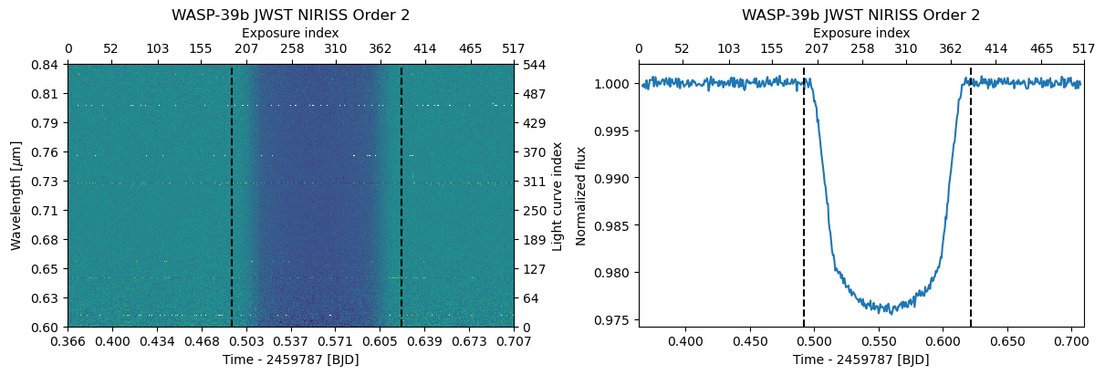
Next, we read the order 2 light curves, remove the strong outliers, and crop the data using the TSData.crop_wavelength method to remove the very noisy red part of the spectrum. After this, we again mask the transit and normalise the light curves. However, this time we can use the order 1 Ephemeris object to set the mask.

[9]:

d2 = read_data('data/nirHiss_order_2.h5', "WASP-39b JWST NIRISS Order 2", noise_group=1, n_baseline=1)
d2.mask_outliers(5)
d2.crop_wavelength(0.6, 0.84)
d2.mask_transit(ephemeris=d1.ephemeris)
d2.normalize_to_poly()

fig, axs = subplots(1, 2, constrained_layout=True)
d2.plot(ax=axs[0])
d2.plot_white(ax=axs[1]);

../../_images/examples_e01_01a_not_so_short_intro_12_0.png

Finalize the dataset#

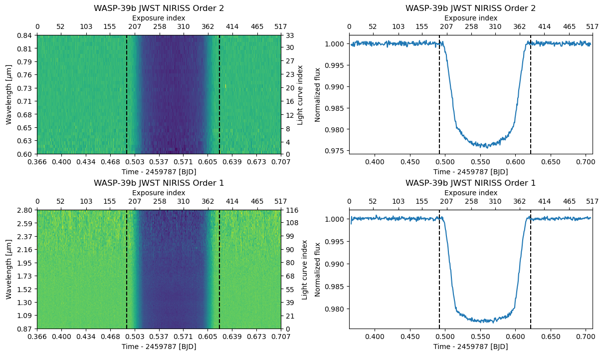
Finally, we bin the spectroscopic light curves to R=100 (we are doing a low-resolution analysis in this notebook anyway) and combine the two orders into a single TSDataGroup object by summing the two TSData objects. We use the estimate_errors=True option to estimate the per-bin flux uncertainties from the data instead of using the error estimates from the pipeline. Now, we end up with a data set consisting of two TSData objects, the first with 56 spectrophotometric light curves covering the wavelength range from 0.57 to 1.00 \(\mu\)m, and the second with 117 light curves covering the wavelength range from 0.87 to 2.83 \(\mu\)m.

Note: The wavelength ranges of the two orders overlap, but this is perfectly fine. Modelling overlapping data sets is an important ability not only when combining orders as here, but also allows the combination of observations with different instruments.

[10]:

db = d2.bin_wavelength(r = 100, estimate_errors=True) + d1.bin_wavelength(r = 100, estimate_errors=True)

fig, axs = subplots(2, 2, figsize=(12, 7), constrained_layout=True)
db.plot(axs=axs[:,0]);
db.plot_white(axs=axs[:,1]);

../../_images/examples_e01_01a_not_so_short_intro_14_0.png

Transmission spectroscopy#

Initialize ExoIris and set the priors#

Now, we’re ready to start the real work! We initialise the ExoIris class by giving it

name: a name for the analysis. This will be used in automatic save files.
ldmodel: a limb darkening model. This can be any limb darkening model accepted by PyTransit’s RoadRunnerModel.
data: a TSData or TSDataGroup object containing the data.
nk: number of radius ratio knots. This sets the final transmission spectrum resolution.
nldc: number of limb darkening knots.
nthreads: number of threads used in the model calculation. We set this to one because we use multiprocessing to parallelise the computations.

[11]:

ts = ExoIris('01a', ldmodel='power-2', data=db, nk=50, nldc=10, nthreads=1)

[12]:

ts.set_radius_ratio_interpolator('bspline-quadratic')

We can take a look at the transmission spectum model parameterization using ExoIris.ps, where ps stands for “parameter set”. Let’s print the first 10 parameters (feel free to print them all to see the full parameterization).

[13]:

ts.ps[:10]

[13]:

[  0 |G| rho            U(a = 0.1, b = 25.0)                     [    0.00 ..      inf],
   1 |G| p              N(μ = 1.0, σ = 1e-05)                    [    0.00 ..      inf],
   2 |G| b              U(a = 0.0, b = 1.0)                      [    0.00 ..      inf],
   3 |G| secw           N(μ = 0.0, σ = 1e-05)                    [   -1.00 ..     1.00],
   4 |G| sesw           N(μ = 0.0, σ = 1e-05)                    [   -1.00 ..     1.00],
   5 |G| tc_00          N(μ = 0.0, σ = 0.1)                      [    -inf ..      inf],
   6 |G| ldc1_00.60334  U(a = 0, b = 1)                          [    -inf ..      inf],
   7 |G| ldc2_00.60334  U(a = 0, b = 1)                          [    -inf ..      inf],
   8 |G| ldc1_00.84668  U(a = 0, b = 1)                          [    -inf ..      inf],
   9 |G| ldc2_00.84668  U(a = 0, b = 1)                          [    -inf ..      inf]]

The parameters are ordered in blocks: [[orbit] [limb darkening] [radius ratio] [white noise multiplier]], where the orbit is always defined by the first six parameters, the number of limb darkening parameters depends on the limb darkening model and number of limb darkening knots, and the number of radius ratios depends on the number of radius ratio knots.

The parameters defining the orbit are:

rho: stellar density [g/cm\(^3\)]
tc: transit center
p: orbital period [d]
b: impact parameter
secw: \(\sqrt e \cos \omega\), where \(e\) is the eccentricity and \(\omega\) is the argument of periastron in radians, set to 0 by default
sesw: \(\sqrt e \sin \omega\), where \(e\) is the eccentricity and \(\omega\) is the argument of periastron in radians, set to 0 by default

The first thing we need to do at the beginning of the analysis is to set priors for the transit centre (tc) and orbital period (p). The stellar density (rho) and the impact parameter (b) are usually constrained well by our photometry, so we can leave the default uninformative priors.

We set the priors using the ExoIris.set_prior method that takes the parameter name as its first argument, the prior as its second argument, and the prior parameters as optional additional arguments. The prior can be any object with logpdf(x) and rvs(n) methods, where x should be allowed to be either a scalar or an array and n an integer, but you can also use shortcut strings for normal priors (NP) and uniform priors (UP).

[14]:

ts.set_prior('tc_00', 'NP', 2459694.286, 0.003)
ts.set_prior('p', 'NP', 4.05487, 1e-5)

[15]:

ts.ps[:10]

[15]:

[  0 |G| rho            U(a = 0.1, b = 25.0)                     [    0.00 ..      inf],
   1 |G| p              N(μ = 4.05487, σ = 1e-05)                [    0.00 ..      inf],
   2 |G| b              U(a = 0.0, b = 1.0)                      [    0.00 ..      inf],
   3 |G| secw           N(μ = 0.0, σ = 1e-05)                    [   -1.00 ..     1.00],
   4 |G| sesw           N(μ = 0.0, σ = 1e-05)                    [   -1.00 ..     1.00],
   5 |G| tc_00          N(μ = 2459694.286, σ = 0.003)            [    -inf ..      inf],
   6 |G| ldc1_00.60334  U(a = 0, b = 1)                          [    -inf ..      inf],
   7 |G| ldc2_00.60334  U(a = 0, b = 1)                          [    -inf ..      inf],
   8 |G| ldc1_00.84668  U(a = 0, b = 1)                          [    -inf ..      inf],
   9 |G| ldc2_00.84668  U(a = 0, b = 1)                          [    -inf ..      inf]]

Set the radius ratio priors#

Next, we can set slightly less uninformative priors on the radius ratios. Let’s take a look at the first four radius ratio parameters.

[16]:

ts.ps[24:30]

[16]:

[ 24 |G| ldc1_02.79341  U(a = 0, b = 1)                          [    -inf ..      inf],
  25 |G| ldc2_02.79341  U(a = 0, b = 1)                          [    -inf ..      inf],
  26 |G| k_00.60334     U(a = 0.02, b = 0.2)                     [    0.00 ..      inf],
  27 |G| k_00.64803     U(a = 0.02, b = 0.2)                     [    0.00 ..      inf],
  28 |G| k_00.69273     U(a = 0.02, b = 0.2)                     [    0.00 ..      inf],
  29 |G| k_00.73742     U(a = 0.02, b = 0.2)                     [    0.00 ..      inf]]

We can set identical priors on all the radius ratio knots using “radius ratios” as the parameter name.

[17]:

ts.set_prior('radius ratios', 'UP', 0.14, 0.15)
ts.ps[24:30]

[17]:

[ 24 |G| ldc1_02.79341  U(a = 0, b = 1)                          [    -inf ..      inf],
  25 |G| ldc2_02.79341  U(a = 0, b = 1)                          [    -inf ..      inf],
  26 |G| k_00.60334     U(a = 0.14, b = 0.15)                    [    0.00 ..      inf],
  27 |G| k_00.64803     U(a = 0.14, b = 0.15)                    [    0.00 ..      inf],
  28 |G| k_00.69273     U(a = 0.14, b = 0.15)                    [    0.00 ..      inf],
  29 |G| k_00.73742     U(a = 0.14, b = 0.15)                    [    0.00 ..      inf]]

Set the noise multiplier priors#

Each TSData object is assigned to a noise group, which has its own white noise multiplier (sigma_mm_xx), which is a free parameter in the fit. The noise multipliers are used to account for underestimated errors, but they have rather narrow priors centred around unity by default.

When creating the TSData objects, we assigned the two data sets to different noise groups by giving them different noise group names. Let’s relax the noise multipliers by giving them all wide uniform priors.

[18]:

ts.ps[75:79]

[18]:

[ 75 |G| k_02.79341     U(a = 0.14, b = 0.15)                    [    0.00 ..      inf],
  76 |G| sigma_m_00     N(μ = 1.0, σ = 0.01)                     [    0.00 ..      inf],
  77 |G| sigma_m_01     N(μ = 1.0, σ = 0.01)                     [    0.00 ..      inf]]

[19]:

ts.set_prior('wn multipliers', 'UP', 0.5, 2.0)
ts.ps[75:79]

[19]:

[ 75 |G| k_02.79341     U(a = 0.14, b = 0.15)                    [    0.00 ..      inf],
  76 |G| sigma_m_00     U(a = 0.5, b = 2.0)                      [    0.00 ..      inf],
  77 |G| sigma_m_01     U(a = 0.5, b = 2.0)                      [    0.00 ..      inf]]

Set the limb darkening priors#

This example uses the power-2 limb darkening model with two limb darkening coefficients per limb darkening knot. Calling ExoIris.set_ldtk_priors calculates the priors for the limb darkening coefficients using LDTk automatically.

Let’s first take a look at the limb darkening coefficient priors for the first two knots before we set the priors:

[20]:

ts.ps[6:10]

[20]:

[  6 |G| ldc1_00.60334  U(a = 0, b = 1)                          [    -inf ..      inf],
   7 |G| ldc2_00.60334  U(a = 0, b = 1)                          [    -inf ..      inf],
   8 |G| ldc1_00.84668  U(a = 0, b = 1)                          [    -inf ..      inf],
   9 |G| ldc2_00.84668  U(a = 0, b = 1)                          [    -inf ..      inf]]

The default prior for the coeffients is a uniform distribution from 0 to 1. Then, lets let’s use LDTk to calculate the priors

[21]:

ts.set_ldtk_prior(teff=(5327, 139), logg=(4.38, 0.09), metal=(-0.01, 0.1), uncertainty_multiplier=10)

And let’s look at the priors now

[22]:

ts.ps[6:10]

[22]:

[  6 |G| ldc1_00.60334  N(μ = 0.733, σ = 0.016)                  [    -inf ..      inf],
   7 |G| ldc2_00.60334  N(μ = 0.812, σ = 0.029)                  [    -inf ..      inf],
   8 |G| ldc1_00.84668  N(μ = 0.597, σ = 0.014)                  [    -inf ..      inf],
   9 |G| ldc2_00.84668  N(μ = 0.697, σ = 0.024)                  [    -inf ..      inf]]

The uncertainty_multiplier parameter inflates the prior uncertainties. This ensures we err on the cautious side when it comes to how much we trust the stellar models that underlie the limb-darkening coefficient priors.

Customise the radius ratio knot locations#

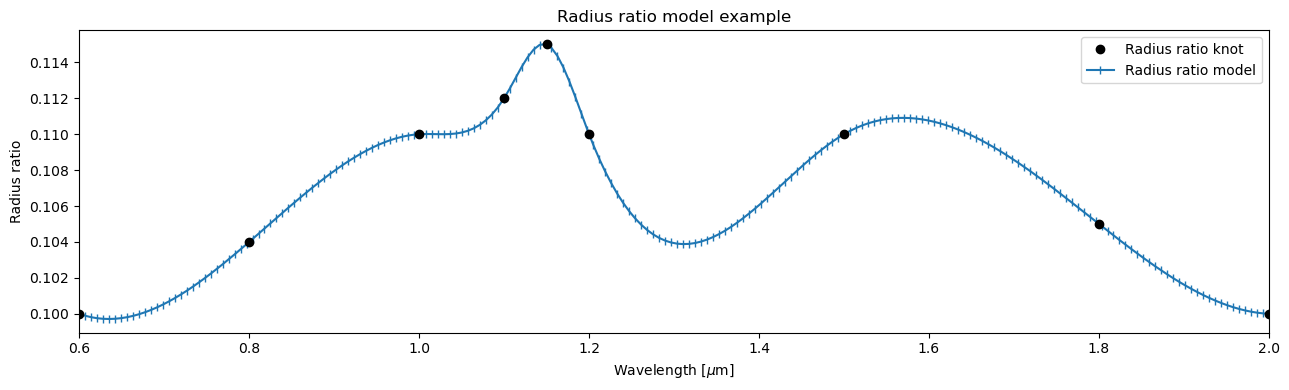
ExoIris represents the planet-to-star radius ratio and the limb darkening parameters as interpolating functions defined by \(N\) points (knots). The wavelength locations of the knots are defined at the start of the analysis (although both the number of knots and knot positions can be modified later), and the knot values are added to the model as free parameters. The spectroscopic transit model is always computed for all wavelength bins in the data, but the number of wavelength bins and the number of radius ratio knots do not need to be the same.

This approach ensures we can optimise the resolution of the transmission spectrum for our science case. For example, we can increase the knot density near strong absorption lines and reduce it in regions where we don’t expect sharp features.

The resolution of the transmission spectrum estimated by ExoIris is defined mainly by two factors:

the wavelength resolution of the data, and
the number and location of the radius ratio knots.

The wavelength resolution of the spectroscopic light curves sets the upper limit for the resolution.

[23]:

fig, ax = subplots(figsize=(13,4))
l = array([0.6, 0.8, 1.00,   1.1, 1.15,   1.2,  1.5, 1.8, 2.0])
k = array([0.1, 0.104, 0.11, 0.112, 0.115, 0.11, 0.11, 0.105, 0.1])
x = linspace(l[0], l[-1], 200)
ax.plot(l, k, 'ko', label='Radius ratio knot', zorder=2)
ax.plot(x, splev(x, splrep(l, k, s=0.0)), '|-', label='Radius ratio model', zorder=1)
ax.legend()
setp(ax, ylabel='Radius ratio', xlabel=r'Wavelength [$\mu$m]', xlim=l[[0,-1]], title='Radius ratio model example')
fig.tight_layout()

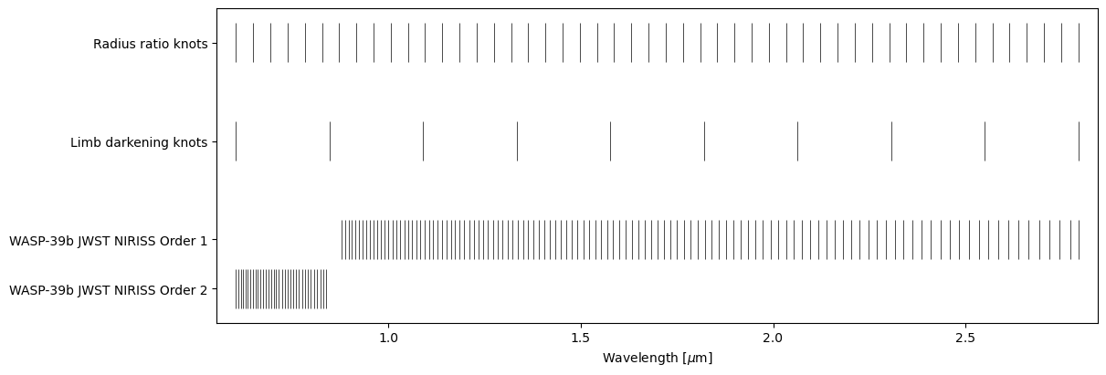
../../_images/examples_e01_01a_not_so_short_intro_38_0.png

ExoIris uses linear spacing between the radius ratio knots by default. The knot locations for the limb darkening parameters and radius ratios can be visualised using the ExoIris.plot_setup method.

[24]:

ts.plot_setup();

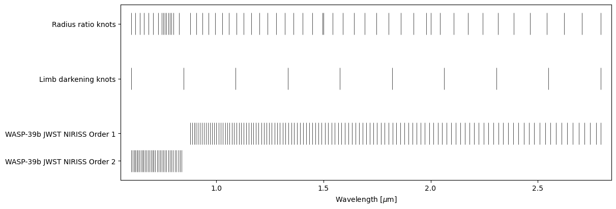
../../_images/examples_e01_01a_not_so_short_intro_40_0.png

Let’s change to use a uniform spacing in log-wavelength (geomspace) and add some extra knots to cover the K line. First, we use ExoIris.set_k_knots to replace the old knots with the new ones, and then we use ExoIris.create_dense_radius_ratio_block to create a block of radius ratio knots using the full data resolution centred around the K line. Finally, we add two random knots using the ExoIris.add_radius_ratio_knots just for fun, and remove a knot that is inside the gap between the two orders. Currently, we don’t have a utility function for the last step, which must be done manually. This changes our number of radius ratio knots (nk) from 50 to 56, and forces ExoIris to change the model parametrisation. The priors for the unaffected parameters are copied, but the new radius ratio knots now have default priors, so we need to set the radius ratio prior again.

[25]:

ts.set_radius_ratio_knots(geomspace(ts.data.wlmin, ts.data.wlmax, 50))
ts.create_dense_radius_ratio_block(0.768-0.025, 0.768+0.025)
ts.add_radius_ratio_knots([1.5, 2.0])

knots = ts.k_knots.copy()
m = (knots > ts.data[0].bbox_wl[1]) & (knots < ts.data[1].bbox_wl[0])
ts.set_radius_ratio_knots(knots[~m])

ts.set_prior('radius ratios', 'UP', 0.14, 0.15)
ts.plot_setup();

../../_images/examples_e01_01a_not_so_short_intro_42_0.png

Fit the white light curve#

Our first fitting step is to fit the white light curve. This is done mainly to obtain accurate estimates for the transit start and end times (T\(_1\) and T\(_4\)) for the baseline normalisation, but it can also give useful insight into whether everything is ok with our data.

[26]:

ts.fit_white()

[27]:

ax = ts.plot_white(figsize=(13,3))

../../_images/examples_e01_01a_not_so_short_intro_45_0.png

Save the model#

We can already save the model for the first time using the ExoIris.save method. This saves the data and the model setup (including the priors) into a fits file that can be later used to recreate the model using the read_model function. We will also call this after the model optimisation and posterior sampling, where the method also saves the optimisation information and the MCMC samples into the fits file.

[28]:

ts.save(overwrite=True)

Set up multiprocessing#

Now we’re almost ready for fitting and MCMC sampling, but since we’re using multiprocessing to parallelise the process, we first need to take some extra steps to make sure everything works the way it’s supposed to.

First, we need to define a log-posterior function that calls the ExoIris log-posterior method. This must be done so that Python can pickle the method for parallelisation (if you know a better way, please let me know). Next, we also create a multiprocessing pool that will be used by the global optimiser and the MCMC sampler.

[29]:

def lnpostf(pv):
    return ts.lnposterior(pv)

pool = Pool(8)

Fit the transmission spectrum#

We start the analysis by fitting the model with the ExoIris.fit method that uses a differential evolution (DE) global optimiser to find the log-posterior mode. The optimiser creates a parameter population of npop parameter vectors and iterates it over niter iterations, where the parameter vector population is clumped closer to the global posterior mode every iteration. The number of iterations and the size of the population depends on the number of radius ratio and limb darkening knots, but we can start with a small number of iterations to see how the minimisation works.

[30]:

ts.fit(niter=25, npop=200, pool=pool, lnpost=lnpostf)

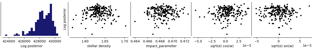
../../_images/examples_e01_01a_not_so_short_intro_51_1.png

The resulting plot shows the distribution of log posterior values for the last parameter vector population, as well as the joint distributions for the log posterior and four model parameters. The fitting should be continued until the log posterior distribution has a width of < 1.

Let’s plot the residuals, transmission spectrum, and the limb darkening parameters corresponding to the best-fitting solution.

[31]:

ts.plot_fit(result='fit', figsize=(13,8), height_ratios=[0.4, 0.6],
            res_args=dict(pmin=5, pmax=95),
            trs_args=dict(xscale='log', ylim=(2.0,2.35), xticks=[0.6, 0.88, 1.16, 1.44, 1.72, 2.0, 2.30, 2.8]));

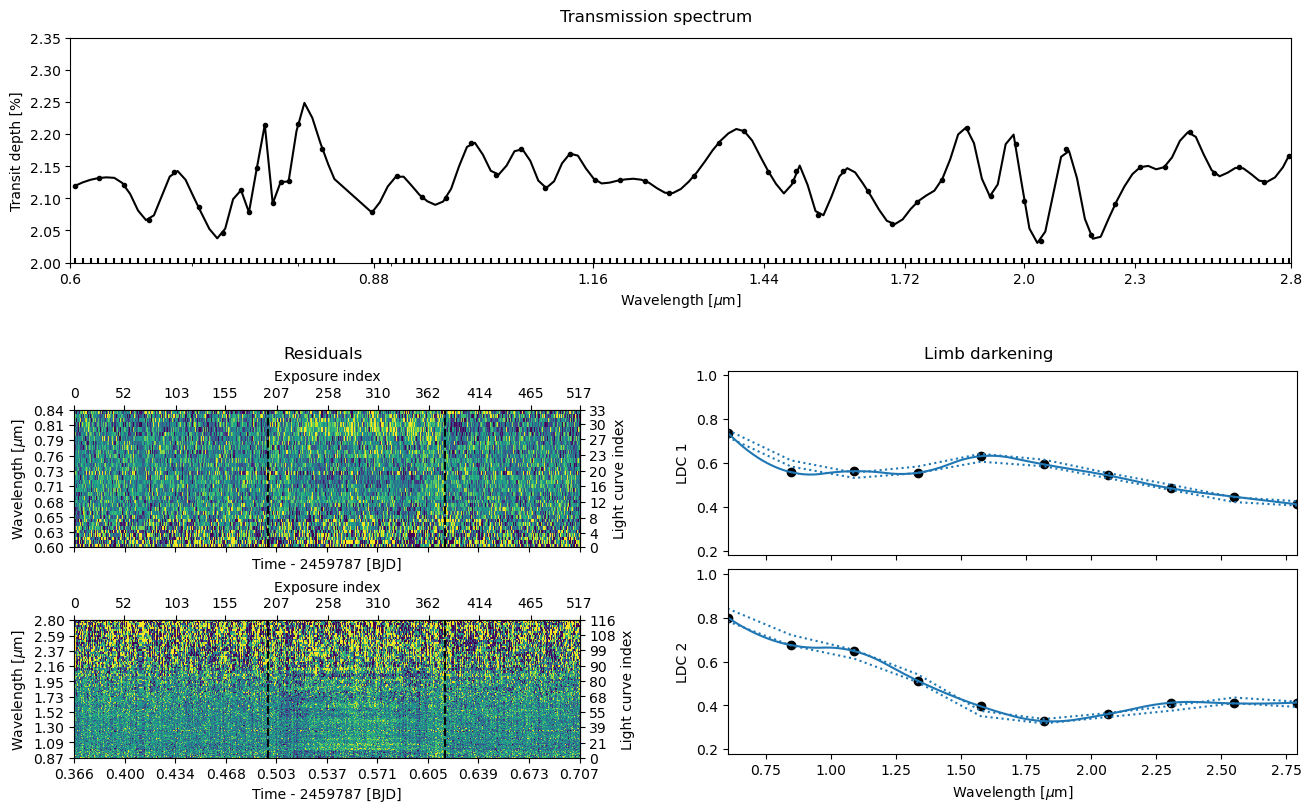
../../_images/examples_e01_01a_not_so_short_intro_53_0.png

We can immediately see from the residual plot that the current best-fit solution is bad. This is something we could have guessed already by looking at the log posterior distribution in the optimiser plot that shows a spread of tens of thousands. Let’s continue the fitting for another 25 iterations. Each successive ExoIris.fit call continues optimisation from the solution of the previous call, and it also plots the old and new posterior and parameter populations at the end of the fit to visualise how the population is changing.

So, it is clear at this stage that running the optimiser for 25 iterations is not doing much. Let’s continue the optimisation for 5000 iterations and see if this does the trick. This should take 2-3 min (or less if you initialise the pool with more processes) and the optimisation should finish before it reaches 5000 iterations (the progress bar turns red).

[32]:

ts.fit(niter=5000, npop=200, pool=pool, lnpost=lnpostf)

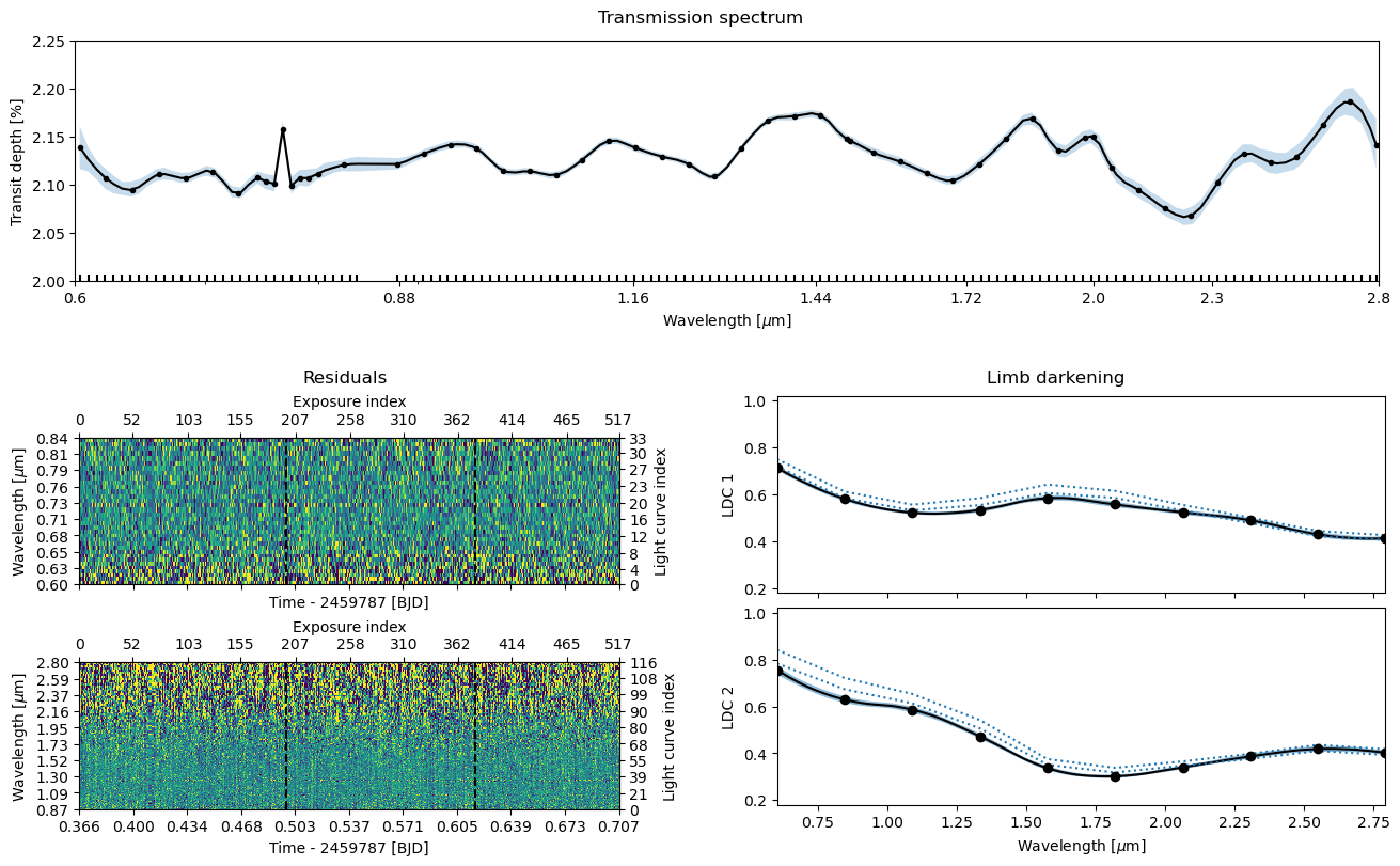
../../_images/examples_e01_01a_not_so_short_intro_55_1.png

Let’s plot everything once again. This time, the residuals look good (there’s no trace of a transit signal there), the transmission spectrum looks something else than just noise, and the limb darkening parameters also look good, so we’re ready to move to the final step: the MCMC sampling.

[33]:

ts.plot_fit(result='fit', figsize=(13,8), height_ratios=[0.4, 0.6],
            res_args=dict(pmin=5, pmax=95),
            trs_args=dict(xscale='log', ylim=(2.0,2.25), xticks=[0.6, 0.88, 1.16, 1.44, 1.72, 2.0, 2.30, 2.8]));

../../_images/examples_e01_01a_not_so_short_intro_57_0.png

Save the optimisation results#

[34]:

ts.save(overwrite=True)

MCMC sampling#

Next comes the final part, obtaining a posterior sample using Markov Chain Monte Carlo (MCMC) sampling. This is done using the ExoIris.sample method, that starts with the parameter vector population from the global optimisation.

As a first step, let’s still inflate the limb darkening parameter prior widths by ten to make sure we’re not constraining them too much in the sampling phase. So, now we set uncertainty_multiplier=100 instead of uncertainty_multiplier=10 that we used in fitting.

[35]:

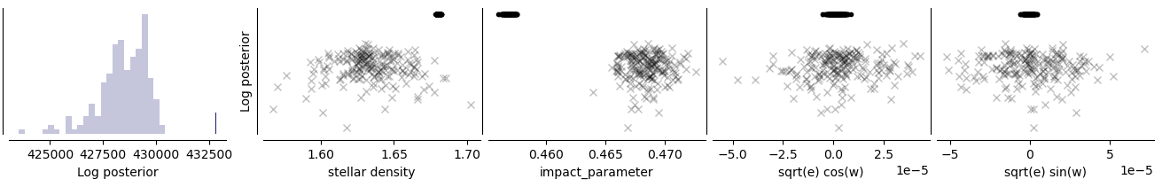
ts.sample(1000, thin=100, repeats=3, pool=pool, lnpost=lnpostf)

[36]:

ts.plot_fit(result='mcmc', figsize=(13,8), height_ratios=[0.4, 0.6],
            res_args=dict(pmin=5, pmax=95),
            trs_args=dict(xscale='log', ylim=(2.0,2.25), xticks=[0.6, 0.88, 1.16, 1.44, 1.72, 2.0, 2.30, 2.8]));

../../_images/examples_e01_01a_not_so_short_intro_62_0.png

Save the results and export the transmission spectrum#

Congratulations, you now have a low-resolution transmission spectrum for your observations! Let’s take a look at this and also save the model one more time to store the posterior samples inside the fits file.

[37]:

ts.save(overwrite=True)

[38]:

ts.transmission_spectrum_table

[38]:

Table length=151

wavelength	radius_ratio	radius_ratio_e	area_ratio	area_ratio_e
um
float64	float64	float64	float64	float64
0.6033383948083351	0.14625606922920667	0.0007465565055328249	0.021390837786500083	0.0002183856298647401
0.6094020972687204	0.14582212887817508	0.0004208705182994625	0.021264093271113435	0.00012273573985220962
0.615526741462376	0.14545926367564438	0.0003411546824640897	0.021158397389061778	9.923263539657539e-05
0.621712939869033	0.14515755440526484	0.000358374508122113	0.021070715601229754	0.00010402867063632245
0.6279613111239981	0.14493559439307274	0.0003136715031786035	0.021006326522074036	9.090411743553368e-05
0.6342724800800181	0.14476719949437425	0.00023968344802599158	0.020957542049448455	6.940581889272982e-05
0.640647077869767	0.14471651490563014	0.0002684935017642936	0.020942869686439033	7.774129247742322e-05
0.6470857419689606	0.14482209352852965	0.0002552685600337906	0.020973438773996878	7.395085713587785e-05
0.653589116260106	0.14504715593278333	0.00019373150332711392	0.021038677444189337	5.62047545402463e-05
...	...	...	...	...
2.585565881504876	0.14645147474707793	0.0003801162344710757	0.021448034455637584	0.00011134945931896678
2.611551468253669	0.14685098851956285	0.00043836603697074264	0.02156521282917665	0.00012875507437085963
2.637798216678329	0.14725965335186209	0.0004275591155482173	0.021685405505685935	0.00012590523342282894
2.6643087515193176	0.14762664225990352	0.00036496925122597235	0.021793625505009042	0.0001077572815456568
2.6910857238963963	0.14784739829071075	0.00045120251360770475	0.0218588531813323	0.00013348976890108837
2.718131811573747	0.14781533055242063	0.0004945348346413827	0.021849371947363243	0.00014627575924371756
2.7454497192277545	0.14754120907814527	0.00045092313422753056	0.021768408376252928	0.0001330752843895203
2.77304217871748	0.14693843436144766	0.0005537883792935183	0.021590903492614708	0.0001627999646094196
2.793411135960404	0.14633142098435353	0.0008774263016267008	0.021412884767423847	0.00025681959644029725

[39]:

pool.close()